The following are computational tools for use with the stretched imaging method as found in the following two references:
MALDI Mass Spectrometric Imaging using the Stretched Sample Method to Reveal Neuropeptide Distributions in Aplysia Nervous Tissue, T.A. Zimmerman, S.S. Rubakhin, E.V. Romanova, K.R. Tucker, Jonathan V. Sweedler, Anal. Chem. 81, 2009, 9402-9409. [PubMed]
Adapting the Stretched Sample Method from Tissue Profiling to Imaging, T. A. Zimmerman, E. B. Monroe, J. V. Sweedler, Proteomics, 8, 2008, 3809-3815. [PubMed]
These tools have been written and validated for a Bruker Ultraflex II MALDI TOF-TOF instrument but can be adapted to other instrumental platforms as needed.
A. Creating Custom Geometry Files
B. Mass Spectra File Conversion
A. Creating Custom Geometry Files
*Note: There is a new more spatially accuracte version of the BeadGeometry software called BeadGeometryMeltedMarkers based on the experimental protocol for geometry file creation found in the newer of the publications, which uses melted holes in the parafilm, as described in T. A. Zimmerman, et al. Anal. Chem. 81, 2009, 9402-9409. [PubMed].
 the BeadGeometryMeltedMarkers application.
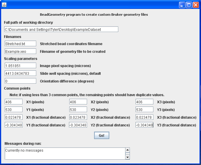
After the program opens, the first parameter accepted by the program is the "Full path of working directory" on the user's local drive that contains all necessary data to run the program.
Alternatively, if the Java JDK is installed, another way to run the program is to compile and run the BeadGeometryMeltedMarkers.java file in a Windows MS-DOS command prompt. After changing to the directory where the java file is saved using the cd command, the commands are as follows:
javac BeadGeometryMeltedMarkers.java [hit Enter]
java BeadGeometryMeltedMarkers [hit Enter]
For creating geometry files using the Bruker TLC geometry with melted markers, needed for acquiring MS/MS images, this software is used: BeadGeometryMeltedMarkersTLCadapter.java. A GUI has also been created:
the BeadGeometryMeltedMarkersTLCadapter application.
the old BeadGeometry application based on detemining scaling with a calibration bar as described in T. A. Zimmerman, E. B. Monroe, J. V. Sweedler, Proteomics, 2008, 8, 3809-3815.
After the program opens, the first parameter accepted by the program is the "Full path of working directory" on the user's local drive that contains all necessary data to run the program.
Alternatively, if the Java JDK is installed, another way to run the program is to compile and run the BeadGeometry.java file in a Windows MS-DOS command prompt. After changing to the directory where the java file is saved using the cd command, the commands are as follows:
javac BeadGeometry.java [hit Enter]
java BeadGeometry [hit Enter]
The stretched sample bead positions are normally identified from a thresholded optical image of the sample using ImageJ software with the Threshold_Colour plugin. Pixel coordinates can be obtained in ImageJ by changing the Analyze-->Set Scale-->Unit of Length parameter to pixel. Using the Analyze-->Analyze Particles command generates a list of bead coordinates. The input text file should consist of the stretched bead X-Y positions in pixel coordinates, in two columns that are delimited by either tabs or spaces. The left column has X-coordinates and the right column has Y-coordinates. For example:
909.167 544.214
782.45 545.8
421.553 549.395
2209.5 549.688
835.845 553.466
...
The Scaling Parameters account for the differences in scaling between the stretched sample image pixels and the Bruker factional-distance coordinate system. The pixel spacing in microns is determined by an image of a calibration bar taken at the same magnification as used to take the stretched sample image. The well spacing parameter does not change and is set as the number of microns equivalent to the distance between spots in the original MTP Slide Adapter II.xeo geometry file, or roughly 0.086957 fractional distance units. One fractional distance unit is equal to 50.8 mm, which is the approximate length of the glass slide. In addition, the rotation angle can be used to rotate the calculated positions to account for differences in orientation between the stretched sample image and the position of the slide in the instrument.
The Common Points are used as points of reference to connect the calculated positions to their corresponding positions in the fractional-distance coordinate system. Multiple separate common points may be used to increase the positional accuracy of the custom geometry file. If less than 3 common points are used, the value for the remaining common point values should be filled in with duplicate values.
Finally, a geometry file is created in the working directory, which should be placed in the "Methods/Geometry Files" folder of the Bruker instrument computer. As the instrument is instructed to take spectra by the AutoXecute function, the new geometry file instructs FlexControl to save spectra in folders that are labeled with the X-Y pixel coordinates of each bead position. These filenames are eventually read into the MSIReconstructor software as the stretched bead positions that are used during the image reconstruction process.
B. Mass Spectra File Conversion
Open mzxmlConvertBatch.m
First, Bruker .fid files are converted into .mzXML files using freely-available Bruker CompassXport software with the -multi command. The -multiName command should name the files as new.mzXML, which is the filename read by the Matlab code used in the subsequent conversion step. The Matlab conversion code requires the Bioinformatics Toolbox to installed be on Matlab. By setting the current directory in Matlab as the root directory that contains all mass spectra, the mzxmlConvertBatch command can be executed from the Matlab Command Window to convert the mass spectra into individual text files that are subsequently read by the MSIReconstructor program. Those text files should be placed in a newly created folder called "Spectra" that exists in the directory where the MSIReconstructor program will run.
C. Image Reconstruction
the MSIReconstructor application.
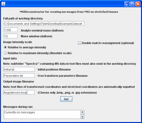
After the program opens, the first parameter accepted by the program is the "Full path of working directory" on the user's local drive that contains all necessary data to run the program.
Alternatively, if the Java JDK is installed, compile and run the MSIReconstructor.java file in a Windows MS-DOS command prompt. After changing to the directory where the java file is saved using the cd command, the commands are as follows:
javac MSIReconstructor.java [hit Enter]
java MSIReconstructor [hit Enter]
There is also a MSIReconstructorMSMS application for plotting MS/MS ion images using the stretched imaging method:
the MSIReconstructorMSMS application.
Alternatively, if the Java JDK is installed, compile and run the MSIReconstructorMSMS.java file in a Windows MS-DOS command prompt.
Open Parameters.txt
Open PlaceDots.java
Open PlaceDots2.java
When run, the MSIReconstructor application will reconstruct an MS image at the nominal mass of the analyte or m/z of interest. The mass window is searched within -value to +value around the nominal analyte mass for the maximum intensity detected within this range. The analyte intensities from individual positions can either be plotted after dividing by the average of the maximum intensity values found in this mass range over all positions, or after dividing by the highest of the maximum intensity values in this mass range over all positions. The latter case produces an image with an absolute intensity scale.
All the text files containing individual spectra should be placed in a new folder called /Spectra, where the MSIReconstructor application automatically searches for these files. The MSIReconstructor application matches the initial bead coordinates to stretched bead coordinates. The stretched bead coordinates are read automatically from the filenames of the spectra-containing text files. The initial positions, however, must be located in a separate text file where the X-Y coordinates are delimited and arranged in a similar manner to the stretched coordinates above.
The parameters text file contains the free transform parameters that are reported by the info palette in Adobe Photoshop, which are used by the MSIReconstructor application in matching the positions. Normally, optical images of the sample both before and after stretching are placed into a new blank Photoshop image file, and the free transform takes place within this file via the Ctrl+T command. The free transform variables are named as follows (all values are in pixels, except for the DeltaADeg value, which is in degrees):
- XCentroidStretched - The X-coordinate at the center of the stretched sample image in the new Photoshop file.
- YCentroidStretched - The Y-coordinate at the center of the stretched sample image in the new Photoshop file.
- XCentroidTransformed - The X-Coordinate at the center of the initial sample image after free transformation.
- YCentroidTransformed - The Y-Coordinate at the center of the initial sample image after free transformation.
- XCenOriginal - The X-Coordinate at the center of the initial sample image before free transformation.
- YCenOriginal - The Y-Coordinate at the center of the initial sample image before free transformation.
- DeltaADeg - The amount of rotation performed during the free transformation.
- WOriginal - The width of the initial sample image before free transformation.
- HOriginal - The height of the initial sample image before free transformation.
- WTransformed - The width of the initial sample image after free transformation.
- HTransformed - The width of the initial sample image after free transformation.
- XCenAloneStretched - The X-coordinate at the center of the stretched sample image.
- YCenAloneStretched - The Y-coordinate at the center of the stretched sample image.
- XCenAloneOriginal - The X-coordinate at the center of the initial sample image.
- YCenAloneOriginal - The Y-coordinate at the center of the initial sample image.
The values in the parameters text file should be tab or space delimited as follows:
XCentroidStretched 1301
XCentroidStretched 1539
...
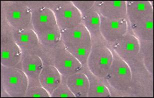
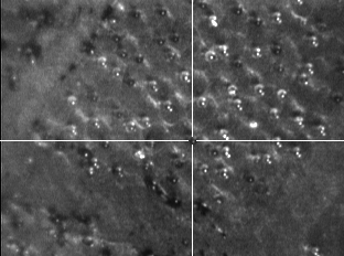
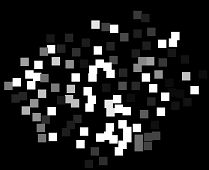
Before the free transformation process, an image file is created using PlaceDots.java that contains small brightly-colored squares at the initial bead positions. This is used in place of the initial sample optical image. Because the initial sample image is enlarged, the apparent size of the beads increases and results in a blurry image. In contrast, the smaller squares help in the free transformation process as they grow more slowly in size and are easier to see, as illustrated in the following image of a free transform overlay.
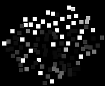
A text file of the stretched image bead coordinates and another file with the calculated transformed bead coordinates are generated during the run. These coordinates can be plotted by compiling and running the PlaceDots2.java program, The resulting image that contains an overlay of the two types of coordinates can be overlaid in a separate layer on top of the image file that contains free transform overlay. Use of the Magic Wand tool in Photoshop removes the dark background from the dots image before visual comparison. This optional exercise is used to visually validate that the calculated transformed positions align with the positions in the free transformed image.
Another optional task can be performed by the MSIReconstructor application. Double match reassignment can reduce matching errors during image reconstruction. If more than one stretched position is matched to a single initial position, the algorithm reassigns one of the positions to the next-nearest unassigned initial position in an iterative fashion. In several validation studies, this reassignment process reproducibly caused a slight improvement in the bead matching rate.
Finally, an ion image is created in either .bmp, .png, or.jpg format that can be converted into Analyze 7.5 format, if necessary, using the Analyze_Writer plugin for ImageJ. There are also several LUT color schemes for visualizing intensity scales under Image-->Lookup Tables in ImageJ.
D. Additional Software
- java JDK is freely available online from Sun Microsystems. See the accompanying installation instructions for help on adding the java CLASSPATH to the environmental variables in Windows.
- ImageJ software is freely available online from NIH. Additionally, the Threshold_Colour and Analyze_Writer plugins for ImageJ are free to download.
- CompassXport is freely available online from Bruker Daltonics under the Service & Support website heading. Free registration is required.
- Matlab and the Bioinformatics Toolbox and are available from The Mathworks.
- Adobe Photoshop is available from Adobe. In addition to the free transform, Photoshop is used for its Photomerge function as stitching together several optical images of the bead sample is often necessary.
E. Example Dataset
Open StretchedImagingExample.zip dataset.
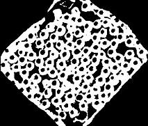
- Open Initial.tif with ImageJ and threshold the image with the Plugins-->Threshold_Colour tool. There is more than one set of thresholding parameters that lead to success. One which works is to modify the a* parameter under CIE lab as a stop filter. The thresholded image looks something like this:
- After thresholding, the image must be converted to 8-bit using Image-->Type-->8-bit.
- The scale must be set to "pixel" in Analyze-->Set Scale--Unit of Length.
- Analyze-->Set Measurements should have centroid selected.
- Analyze-->Analyze Particles with 0.8 circularity gives about 114 coordinates. It is useful to select Show-->Outlines to view the coordinates that were found by ImageJ. If running the Analyze Particles command more than once for optimization purposes, the Results window should be closed in between each run as coordinates from each run are concatenated onto the file. The Results file can be saved with a .xls extension for opening in Microsoft Excel, which will allows trimming of extra columns of data before saving the file as a .txt file. The initial coordinates file should look something like this file: Initial.txt.
- The sample is manually stretched, and optical images of the stretched sample are taken.
- Open Stretched.tif with ImageJ and threshold this image in the same manner as the initial sample image, repeating steps 1-5. Thresholding is generally much easier on stretched sample optical images because the beads are not touching each other. This gives approximately 111 coordinates and should be in a file similar to the following: Stretched.txt.
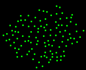
- Before creation of the geometry file, it is useful to do the free transformation to see if image reconstruction will be successful for the sample. Create a file of colored squares at each of the initial bead positions using PlaceDots.java, or use this file: InitialDots.bmp.
- Open Stretched.tif in Photoshop and press Ctrl + T to identify the X-Y pixel coordinates of its centroid, which are X = 474 and Y = 353. Place these in the Parameters.txt file.
- Copy Stretched.tif and place it along with a copy of the InitialDots.bmp file into a blank Photoshop file that is at least large enough to contain both images. The initial dots image should be in a higher layer than the stretched sample image. Use the Magic Wand tool in Photoshop to remove the black background from the initial dots image. Take note of the centroid positions of each image and the width/height of the initial dots image using the Ctrl + T command and Info Palette and record these in the Parameters.txt file.
- Select the initial dots image, press Ctrl + T and change the position, width, height, and rotation angle of this image until it overlays the stretched sample image such that the beads are correctly matched by proximity. Record the final parameters of the transformed image in the Parameters.txt file, which should now look something like this.
- To create the geometry file, the calibration bar is measured. Open CalibrationBar.tif in ImageJ and manually measure the length between two corners of the bar that are separated by a longer side. Analyze-->Set Scale reports a distance of approximately 540 pixels. The pixel spacing in microns is then: 1000/540 = 1.851851 microns/pixel.
- Upon loading the sample into the Bruker Ultraflex II instrument, there is little or no rotation angle difference between the orientation of the sample in the FlexControl window and the sample image, so 0 degrees is appropriate.
- One of the points in the MTP Slide Adapter II.xeo file was adjusted to read X = 0.023478 and Y = -0.304348, which falls directly in the area of the sample as shown below in a photo of the FlexControl window.
- Open Stretched.tif and verify that this point visually corresponds to pixel coordinates X = 406 and Y = 530.
- Entering all of these parameters into the BeadGeometry application should look like this image and the final geometry file should look something like this which can be viewed in notepad: Example.xeo. When the sample was loaded into the Bruker instrument, along with the geometry file, data was taken exclusively from the bead positions.
- Open an MS-DOS command prompt and change to the root folder containing all mass spectra. Use the CompassXport -multi command, with -multiName set to new.mzXML, which creates mzXML files.
- Open Matlab and add mzxmlConvertBatch.m to the Matlab path, File-->Set Path. Change to the root folder containing all spectra and execute the "mzxmlConvertBatch" command. This creates spectra-containing text files in the root directory that should be placed in a folder called "Spectra" which should in turn be placed in the working directory where MSIReconstructor is to be run.
- The MSIReconstructor panel should be filled out in a manner similar to this photo. After creating ion images for the both Ang I and Ang II peptides, their chemical distributions appear to match the color distributions of the initial sample optical image. Clear beads were coated with Ang I and generally appear in the center of the sample, while blue beads were coated with Ang II and generally appear on the edges of the sample.
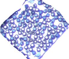
Initial sample optical image
| 
| 
|
